Question
State and explain law of supply with exceptions.
Law of Supply :
(A) Introduction : The law of supply was introduced by Dr. Alfred Marshall in his book “Principles of Economics” published in 1890. The law establishes a functional relationship between the price of a commodity and quantity supplied of that commodity. It explains the general tendency of the sellers in offering more goods for sale at a higher price than at a lower price.
(B) Statement of the Law : According to Prof. Alfred Marshall “Other things remaining constant, the higher the price of the commodity, greater is the quantity supplied and lower the price of the commodity, smaller is the quantity supplied.”In other words, quantity supplied of a commodity varies directly with price i.e., with a fall in price supply contract and with a rise in price supply expands.
S = f (P) [S = Supply, P = Price, f = Function of]
The law can be better understood with the help of a market supply schedule and market supply curve.
(C) Market Supply Schedule : Market supply schedule is a tabular representation of various quantities of a commodity offered for sale by all the sellers in the market at different prices during a given period of time. The schedule is a hypothetical one except one price rest are imaginary prices.
The above schedule clearly shows that sellers in general want to sell more at high prices and less at low price. E.g., at a low price of Rs.10 per unit the seller supplies only 100 units per day and at high price of Rs. 50 the supply rises to 500 units of ‘X’ per day.
(D) Market Supply Curve : It is graphical representation of the above market supply schedule. Price is measured on ‘Y’ axis and quantity supplied on ‘X’ axis and above schedule is plotted. We derive a supply curve SS.
Market Supply Schedule
| Price of ‘X’ per unit (in ?) | Total Market Supply per day (in units) |
| 10 | 100 |
| 20 | 200 |
| 30 | 300 |
| 40 | 400 |
| 50 | 500 |
There are some exceptions to the law of s supply. Following are such cases when supply may fall with the rises in price or rise with the fall in price.
(1) Labour supply : Supply of labour in the ) terms of hours of work is an important exception pointed out by economists. Generally when wages rise, workers work more, but after a certain point if wages continue to rise, supply of labour falls i.e. workers wish to earn more by work in for less hours and supply curve of labour would bend backwards as shown below :
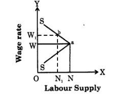
In this figure as wage rate rises up to 0W, ;i supply of labor also rises up to ON, but when wage rate rises to 0W., labour supply falls from ON to 0Nr Hence an exception.
(2) Saving : In case of savings generally it is observed that as the rate of interest rises, savings also rises but some people want to have a fixed regular income by way of interest. They may save less at a higher rate of interest and save more at a lower rate of interest. For example : suppose a person is interested in earning a fixed income of ₹ 800 p.a. then he saves ₹ 10,000/- at 8% rate of interest but when rate of interest increases to 10%, he will save only ₹ 8,000/-.
(3) Future Expectations: If the seller expects a fall in price in future, then he will supply more today even at a low price. But if he expects the prices to rise further in future he will withhold the supply today to supply more in future at a high price.
(4) Need for Cash : When the sellers are in urgent need of liquid cash, then even at a lower price they will offer more goods for sale.
(5) Rare Goods : In case of rare collections such as rare painting, old coins, antique, the law is not applicable as the supply remains fixed. The supply curve is a vertical straight line parallel to Y axis.
(6) Agricultural Goods: Supply of agricultural product is influenced by natural factors like climatic conditions, rainfall etc., which cannot be controlled by man. So in bad weather condition, even at a higher price the supply of agricultural commodities will not increase.
Generate a complete, print-ready paper with questions like this in minutes — across 16+ boards, with answer keys.
India’s Merchandise Trade (US $ Billion)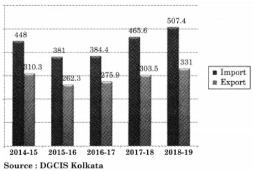
QU 1. In the above bar diagram during which year export was maximum and how much was it?
QU 2. In which year import was maximum and how much was it?
QU 3. In which year import was least and how much was it?
QU 4. Find out the trade deficit in the year 2017-18?
QU 5. How much is the export increase in the year 2018-19 as compared to 2014-15?
QU 6. How much is the import increase in the year 2018-19 as compared to 2017-18?
QU 7. Express your views on India’s merchandise trade.