Question
What is ‘effective demand’? How will you derive the autonomous expenditure multiplier when price of final goods and the rate of interest are given?

Answer

Aggregate demand at the point of equilibrium is called an effective demand, because it becomes effective in determining national income. It is the level of demand which is fully met by corresponding supply with no tendency to expand or contract. Thus effective demand is the amount which is actually spent. In Keynesian framework which deals in short run analysis, equilibrium level of income and employment are determined solely by level of aggregate demand (i.e., effective demand) because aggregate supply (or national income) is assumed to be given and constant. Also because in the short run physical and technical conditions affecting aggregate supply do not often change. So it is the level of effective demand or AD which influences the level of output, income and employment. Thus for increasing the level of income, increase in effective demand is essential. In short, AD holds the key to the full employment level of income. The concept of effective demand can be explained with the help of the given diagram.

The x-axis represents income/ output level and y-axis represents the level of aggregate demand. E is the equilibrium point where the two curves AS and AD meet. EG is the effective demand and output level is determined by AD (assuming the elasticity of supply to be perfectly elastic).

Autonomous expenditure multiplier is derived as:

Y = AD (at equilibrium)

Y = A + cY [Where AD = A + cY]

Y - cY = A

Y (1 - c) = A

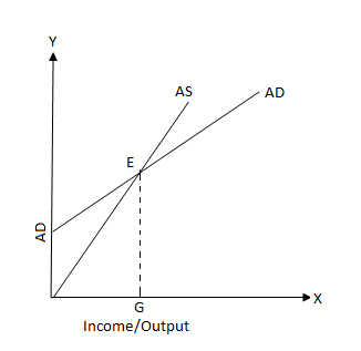
$\text{Y}=\frac{\text{A}}{1-\text{c}}$

Where,

A = Autonomous expenditure

c = MPC

Y = level of income

$\frac{1}{1-\text{c}}=$ autonomous expenditure multiplier.

So, the autonomous expenditure multiplier is dependent on the income and MPC.

Need a full question paper?

Generate a complete, print-ready paper with questions like this in minutes — across 16+ boards, with answer keys.

Start Generating Free

Similar questions

Explain the concepts of the short run and the long run.
What are the different phases in the Law of Variable Proportions in terms of marginal product? Give reason behind each phase. Use diagram.
Explain the concepts of Opportunity Cost and Marginal Rate of Transformation using a production possibility schedule based on the assumption that no resource is equally efficient in production of all goods.
In the above example, if exports change to X = 100, find the change in equilibrium income and the net export balance.
When price of a commodity X falls by 10 percent, its demand rises from 150 units to 180 units. Calculate its price elasticity of demand. How much should be the percentage fall in its price so that demand rises from 150 to 210 units?
Explain the implications of the following:
  1. Product differentiation in monopolistic competition.
  2. Perfect knowledge in perfect competition.
The equilibrium level of income in an economy is ₹ 1,000 crore. The autonomous consumption expenditure is equal to ₹ 100 crore and investment expenditure ₹ 500 crore.

Calculate:

  1. Consumption expenditure at equilibrium level of national income,
  2. Marginal Propensity to save,
  3. Saving Function;
  4. Break-even level of Income.
Calculate 'Net Domestic Product at Factor Cost' and 'Gross National Disposable Income':
 
 
(Rs. Crores)
(i)
Net current transfers to abroad
15
(ii)
Private final consumption expenditure
800
(iii)
Net imports
(-)20
(iv)
Net domestic capital formation
100
(v)
Net factor income to abroad
10
(vi)
Depreciation
50
(vii)
Change in stocks
17
(viii)
Net indirect tax
120
(ix)
Government final consumption expenditure
200
(x)
Exports
30
Assuming that increase in investment is Rs. 1000 crore and marginal propensity to consume is 0.9, explain the working of multiplier.
Explain the following functions of the central bank:
  1. Bank of issue
  2. Bankers' bank